Quick start

In the two quick-start examples, roots are generated without biological relevance (standard lateral root length can’t be longer than the bearing axis remaining branching length ). Notebook examples give examples on realistic architecture.

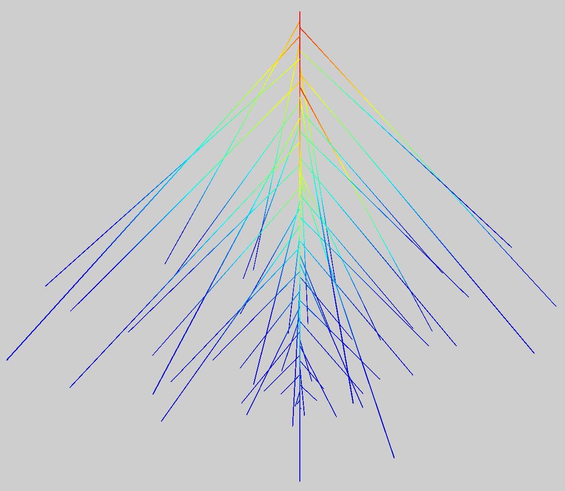
Generating a root

Build a root and display it in the PlantGL viewer.

from openalea.hydroroot.main import root_builder
from openalea.hydroroot.display import plot
g, primary_length, total_length, surface, seed = root_builder(order_max=1)
plot(g)

Hydraulic simulation

Build a root, run the hydraulic solver and display the eat map representation of the incoming local radial flows on an arabidopsis root in the PlantGL viewer.

from openalea.hydroroot.main import hydroroot
from openalea.hydroroot.display import plot
K = ([0,0.2],[0.0,1.0e-2])
k = ([0.0,0.2],[300.0,300.0])
g, surface, volume, Keq, Jv_global = hydroroot(axial_conductivity_data = K, radial_conductivity_data=k, order_max = 1)
plot(g, prop_cmap = 'j')

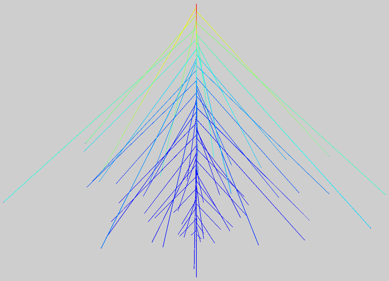
K (\(10^{-9}\ m^4.s^{-1}.MPa^{-1}\)) and k (\(10^{-9}\ m.s^{-1}.MPa^{-1}\)) are the axial and radial conductances, versus distance to tip (m), respectively.

Notebook examples

See examples in the Gallery that illustrate some HydroRoot capabilities.

See also the jupyter notebook boursiac2022.ipynb in example/Bourisac2022 that is aimed to run different simulations to generate figures and tables of Bourisac et al. 2022 [boursiac2022].