
Example of cut and flow (CnF) analysis#
The purposes here are:
to show how to use the
cut_and_flowfunctions allowing tha analysis of CnF experimentsto illustrate how it is important to consider water and solutes transport in some water stress cases to avoid significative error on hydraulic parameters.
CnF experiment protocol is described in Boursiac et al.. In this work, experiments were performed on Arabidopsis in control condition only therefore analysis was done with the pure water solver of HydroRoot. A second publication, Bauget et al. 2023 was focused on the phenotypage of maize roots under water stress. The authors showed that in this condition solute transport had to be accounting for CnF analysis.
Inputs#
There are 3 kinds of input files:
a yaml file with general and mandatory parameters see documentation for details, or example of files in the
exampledirectory that are well commented.a
csvfile with CnF data mandatory for any CnF analysis, for exampleexample/data/maize_cnf_data.csv.a
csvfile with flux vs pressure (JvP) needed only with the solute-water solver, for exampleexample/data/maize_JvP_data.csv.
cnf_data.csv#
csv file containing data of cut and flow data of with the following columns:
arch: sample name that must be contained in the ‘input_file’ of the yaml file
dP_Mpa: column with the working cut and flow pressure (in relative to the base) if constant, may be empty see below
J0, J1, …, Jn: columns that start with ‘J’ containing the flux values, 1st the for the full root, then 1st cut, 2d cut, etc.
lcut1, …., lcutn: columns starting with ‘lcut’ containing the maximum length to the base after each cut, 1st cut, 2d cut, etc. (not the for full root)
dP0, dP1,.., dPn: column starting with ‘dP’ containing the working pressure (in relative to the base) of each steps (if not constant): full root, 1st cut, 2d cut, etc.
JvP_data.csv#
csv file containing data of Jv(P) data of with the following columns:
arch: sample name that must be contained in the ‘input_file’ of the yaml file
J0, J1, …, Jn: columns that start with ‘J’ containing the flux values of each pressure steps
dP0, dP1,.., dPn: column starting with ‘dP’ containing the working pressure (in relative to the base) of each steps
Complements#
CnF experiments and analysis with pure water solver (
parameters.ymlandcnf_data.csvinputs), see Boursiac et al..CnF experiments and analysis with solute-water solver (
parameters.yml,cnf_data.csvandJvP_data.csvinputs), see Bauget et al. 2023.modeling principles in HydroRoot documentation.
This notebook calls python scripts calling the wapper functions.
[8]:
import warnings
warnings.filterwarnings('ignore')
Maize root in control condition#
Solute solver#
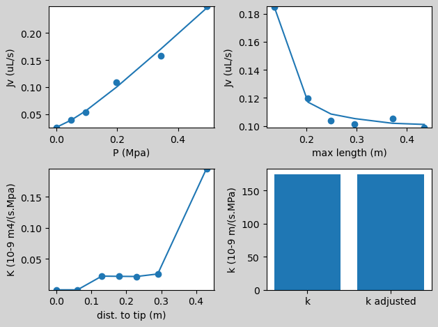
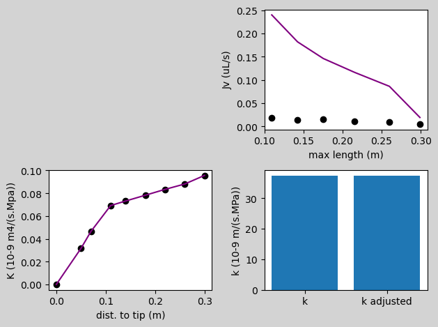
Here an example of a maize root with measurements done in hydroponic solution (control), in the parameters file parameters_Ctr-3P2.yml hydraulic and solute transport parameters have been already optimized to get the best fit (lines in the plots) of data (dot).
[9]:
%run example_cut_and_flow_water_solute.py parameters_Ctr-3P2.yml
running time is 3.079962730407715
With hydrostatic solver#
Here we run simulation with the same input parameter file with the hydrostatic solver (no solute transport).
[10]:
%run example_cut_and_flow_pure_water.py parameters_Ctr-3P2.yml
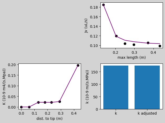
We can note that the fit of data is not as good as simulation with water-solute solver.
We then adjust K and k with hydrostatic solver to fit data. It takes around 40 s.
[11]:
%run example_cut_and_flow_pure_water.py parameters_Ctr-3P2.yml -op -v
*********** pre_optimization ************************
pre-optimization ar: 9.34e-01
pre-optimization ax: 1.01e+00
****************************************************************
finished minimize K: [ 2.99e-04, 7.19e-04, 3.17e-03, 3.17e-03, 5.07e-03, 5.85e-02, 1.43e-01 ]
finished minimize k0: , 1.63e+02
          plant  cut length (m)  max_length  k (10-9 m/s/MPa)  length (m)  surface (m2)  Jv (uL/s)  Jexp (uL/s)
0  Exp03_P2.txt          0.0000      0.4340        163.141792       3.979      0.005644   0.101705     0.098667
1  Exp03_P2.txt          0.0623      0.3717        163.141792       3.915      0.005432   0.101730     0.105333
2  Exp03_P2.txt          0.1374      0.2966        163.141792       3.829      0.005172   0.102061     0.101444
3  Exp03_P2.txt          0.1847      0.2493        163.141792       3.694      0.004912   0.103611     0.103667
4  Exp03_P2.txt          0.2305      0.2035        163.141792       3.468      0.004547   0.119508     0.119500
5  Exp03_P2.txt          0.2982      0.1358        163.141792       2.947      0.003785   0.184774     0.184778
      x     K 1st  K optimized
0  0.00  0.000230     0.000299
1  0.06  0.000227     0.000719
2  0.13  0.022300     0.003172
3  0.18  0.021960     0.003172
4  0.23  0.021720     0.005069
5  0.29  0.025770     0.058471
6  0.43  0.195400     0.142783
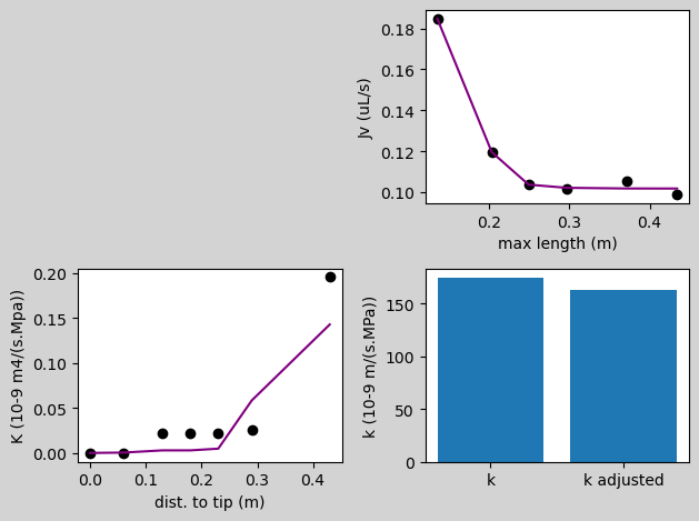
We can note that there are no significant differences between hydraulic parameters from water-solute and pure water solver in control condition.
Maize root in control condition#
Solute solver#
Here an example of a maize root with measurements done in a PEG solution (150 g/l) simulating water stress, in the parameters file parameters_150-5P13.yml hydraulic and solute transport parameters have been already optimized to get the best fit.
[12]:
%run example_cut_and_flow_water_solute.py parameters_150-5P13.yml
running time is 1.745145320892334
With hydrostatic solver#
[13]:
%run example_cut_and_flow_pure_water.py parameters_150-5P13.yml
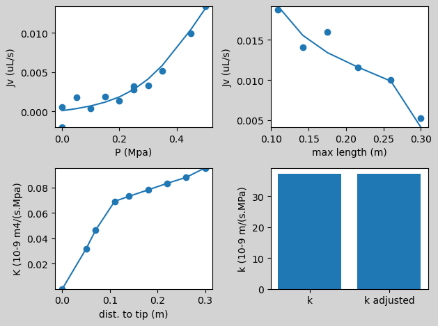
Here the fit is very bad. Let’s adjust parameters with the hydrostatic solver to fit the data. It takes around 13 s.
[14]:
%run example_cut_and_flow_pure_water.py parameters_150-5P13.yml -op -v
*********** pre_optimization ************************
pre-optimization ar: 3.95e-01
pre-optimization ax: 7.70e-02
****************************************************************
finished minimize K: [ 1.71e-07, 3.58e-03, 4.49e-03, 6.54e-03, 6.54e-03, 6.54e-03, 6.54e-03, 6.54e-03, 6.54e-03 ]
finished minimize k0: , 1.40e+01
finished minimize K: [ 2.17e-08, 3.74e-03, 4.66e-03, 6.61e-03, 6.61e-03, 6.61e-03, 6.61e-03, 6.61e-03, 6.61e-03 ]
finished minimize k0: , 1.40e+01
           plant  cut length (m)  max_length  k (10-9 m/s/MPa)  length (m)  surface (m2)  Jv (uL/s)  Jexp (uL/s)
0  Exp05_P13.txt        0.000000    0.299000         14.012456       0.954      0.001796   0.005817     0.005282
1  Exp05_P13.txt        0.039098    0.259902         14.012456       0.913      0.001663   0.009844     0.009976
2  Exp05_P13.txt        0.083459    0.215541         14.012456       0.869      0.001521   0.011526     0.011560
3  Exp05_P13.txt        0.123762    0.175238         14.012456       0.829      0.001392   0.013332     0.015949
4  Exp05_P13.txt        0.156760    0.142240         14.012456       0.772      0.001255   0.015562     0.014115
5  Exp05_P13.txt        0.189835    0.109165         14.012456       0.680      0.001073   0.019297     0.018726
      x     K 1st   K optimized
0  0.00  0.000019  2.171835e-08
1  0.05  0.031690  3.735261e-03
2  0.07  0.046450  4.660776e-03
3  0.11  0.069210  6.613485e-03
4  0.14  0.073150  6.614899e-03
5  0.18  0.078230  6.614899e-03
6  0.22  0.083380  6.614899e-03
7  0.26  0.088110  6.614899e-03
8  0.30  0.095630  6.614899e-03
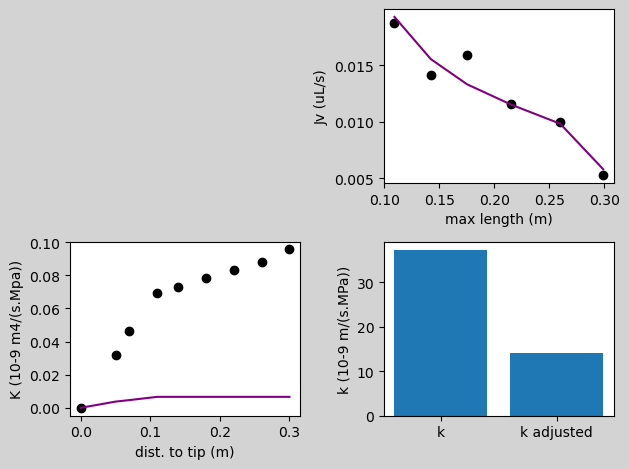
Therefore without taking account for solute transport we make an error of 62 % on k and 93 % on the max of K
[ ]: